텐서플로우 공식 가이드 중 Neural machine translation with attention 문서의 실습을 참고하였습니다.
Neural machine translation with attention
스페인어에서 영어로 기계번역을 수행하는 seq2seq 모델을 직접 구현해본다.
기본적인 데이터의 처리 과정은 이전과 같다. 전처리 과정은 생략하고 실제 인코더-어텐션-디코더를 클래스 형태로 구현하는 부분의 코드를 분석해본다.
Encoder 1. 클래스 설계 1 2 3 4 5 6 7 8 9 10 11 12 13 14 15 16 17 18 class Encoder (tf.keras.Model ): def __init__ (self, vocab_size, embedding_dim, enc_units, batch_sz ): super (Encoder, self).__init__() self.batch_sz = batch_sz self.enc_units = enc_units self.embedding = tf.keras.layers.Embedding(vocab_size, embedding_dim) self.gru = tf.keras.layers.GRU(self.enc_units, return_sequences=True , return_state=True , recurrent_initializer='glorot_uniform' ) def call (self, x, hidden ): x = self.embedding(x) output, state = self.gru(x, initial_state = hidden) return output, state def initialize_hidden_state (self ): return tf.zeros((self.batch_sz, self.enc_units))
[기본 파이썬 문법]
class Encoder(tf.keras.Model) : Encoder 클래스는 tf.keras.Model 클래스를 상속
__ init __ : 클래스 생성자. 객체 생성 시점에 자동 호출
super(Encoder, self).__ init __() : 부모 클래스 초기화. super()와 super(A, self)의 차이점 참고
[코드 분석]
2. 사용 1 2 3 4 5 6 7 encoder = Encoder(vocab_inp_size, embedding_dim, units, BATCH_SIZE) sample_hidden = encoder.initialize_hidden_state() sample_output, sample_hidden = encoder(example_input_batch, sample_hidden) print ('Encoder output shape: (batch size, sequence length, units) {}' .format (sample_output.shape))print ('Encoder Hidden state shape: (batch size, units) {}' .format (sample_hidden.shape))
3. 코드분석 - Embedding layer의 통과 위의 코드는 이전의 전처리를 수행해야 시행해볼 수 있다. 바로 인코더 모델의 모습만 확인해 볼 수 있도록 임의의 텐서를 만들어 모델 구조를 확인해보자.
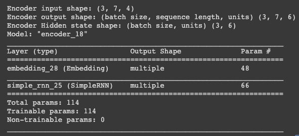
1 2 3 4 5 6 7 8 9 10 11 12 13 14 15 16 17 18 19 20 21 22 23 24 25 26 27 28 29 30 31 import tensorflow as tfclass Encoder (tf.keras.Model ): def __init__ (self, vocab_size, embedding_dim, enc_units, batch_sz ): super (Encoder, self).__init__() self.batch_sz = batch_sz self.enc_units = enc_units self.embedding = tf.keras.layers.Embedding(vocab_size, embedding_dim) self.rnn = tf.keras.layers.SimpleRNN(self.enc_units, return_sequences=True , return_state=True , recurrent_initializer='glorot_uniform' ) def call (self, x, hidden ): x = self.embedding(x) print ('Encoder input shape: {}' .format (x.shape)) output, state = self.rnn(x, initial_state = hidden) return output, state def initialize_hidden_state (self ): return tf.zeros((self.batch_sz, self.enc_units)) example_input_batch = tf.zeros((3 , 7 )) encoder = Encoder(12 , 4 , 6 , 3 ) sample_hidden = encoder.initialize_hidden_state() sample_output, sample_hidden = encoder(example_input_batch, sample_hidden) print ('Encoder output shape: (batch size, sequence length, units) {}' .format (sample_output.shape))print ('Encoder Hidden state shape: (batch size, units) {}' .format (sample_hidden.shape))encoder.summary()
위의 코드는
단어집합 크기 : 12
임베딩 차원 : 4
은닉상태의 크기 : 6
배치크기 : 3
인 경우이다. 이때 입력 배치는 (3, 7)의 텐서이다. 공부를 하면서 헷갈리는 부분이 있어서 텐서의 크기를 단어집합 크기와 동일하게 3, 12로 잡고 싶었는데 그렇게 하면 out of bound 인덱스 오류가 나더라. 즉, 모델의 단어집합 크기와 동일한 크기의 텐서를 초기 입력으로 넣을 수 없는 듯 하다. 어쩔 수 없이 만든 그림은 (1) 모델의 단어집합 크기가 12인 경우 모델의 모습 과 (2) 모델의 초기 입력 텐서의 크기가 (3(=batch_sz), 12)인 경우 두개의 짬뽕이 되어버림.
위의 코드를 시행하면 아래의 결과가 나온다.
임베딩 레이어
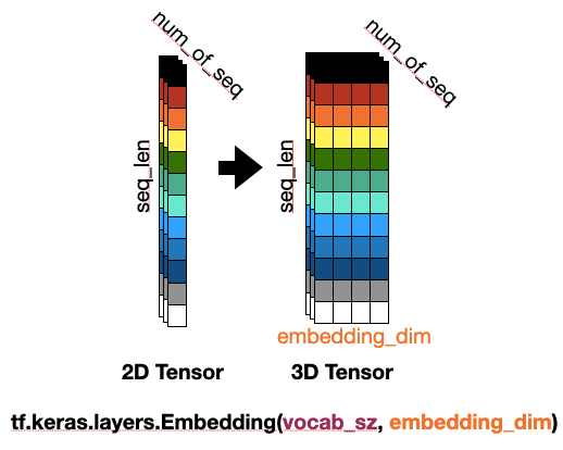
케라스의 Embedding 함수는 단어집합의 크기와 임베딩 차원을 변수로 받아 임베딩 레이어를 만들어준다. 이때 레이어에 모델을 추가하는 것과 모델에 들어가는 텐서는 별도이다. 난 이 개념을 이해하는게 넘나 어려웠다..ㅋㅋㅋㅠ
이게 뭔말인고 하니… 위의 그림은 시퀀스 길이가 12, 시퀀스 개수가 3, 임베딩 차원이 4인 경우 Embedding Layer를 통과했을때 텐서의 크기변환 시각화이다.
즉, 아래와 같은 예시가 있다고 가정하자.
[[I, am, studying, neural, language, machine, translation, in, a, cafe, near, home], [I, am, studying, language], [neural, machine, translation]]
이때 각 시퀀스를 12의 길이로 패딩해주자.
[ [I, am, studying, neural, language, machine, translation, in, a, cafe, near, home],
[I, am, studying, language, , , , , , , , ],
[neural, machine, translation, , , , , , , , , ]]
패딩된 시퀀스를 정수 인코딩해주면 대충 아래처럼 된다.
[[1, 2, 3, …, 12], [1, 2, 3, 5, 0, 0, … 0], [4, 6, 7, 0, 0….. 0]]
= 크기 (3, 12)
그럼 이 (3, 12)의 텐서가 Embedding(단어집합 크기, 임베딩차원) 으로 만들어진 임베딩 레이어에 들어가는거다.
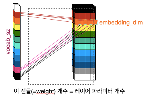
이때 단어집합의 크기를 14라고 하면(단어장 개수 + + ) 해당 텐서가 들어가는 임베딩 레이어 모델 에는 임베딩 작업을 위한 룩업 테이블 이 생성되고, 이때 이 룩업테이블의 크기는 임베딩 레이어의 파라미터의 개수 가 된다.
num of parameters in Embedding layer 14(vocab sz) * 4(embedding dim)
위의 코드에서는 example_input_batch가 입력으로 들어가는데 코드 설명을 보면 (64, 16)의 크기이며 단어장 크기는 9000정도라고 한다. 또한 임베딩 차원은 256이라고 한다.
그럼 결국 다음과 같다.
길이가 16인 시퀀스가 64개 있다. : 16개의 단어로 이뤄진 문장이 64개
(64, 16)인 이 입력텐서는 임베딩 레이어를 거치면 (64, 16, 9000) 이 된다.
임베딩 레이어의 파라미터 개수는 9000 * 256
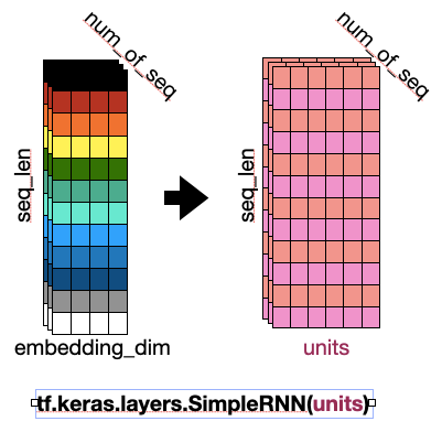
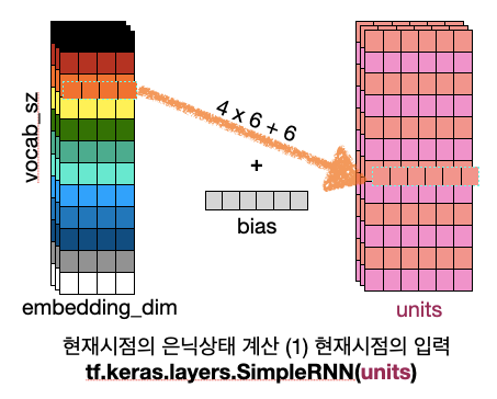
4. 코드분석 - RNN 은닉층의 통과 원본 코드에서는 GRU를 사용했지만 보다 용이한 (나의)이해를 위해 사용하는 은닉층을 SimpleRNN으로 변경해보았다.
아까 위에서 임베딩 층을 통과하면서 (시퀀스 개수, 시퀀스 길이, 임베딩 차원) 으로 변환된 텐서는 RNN의 입력으로 들어가게 된다.
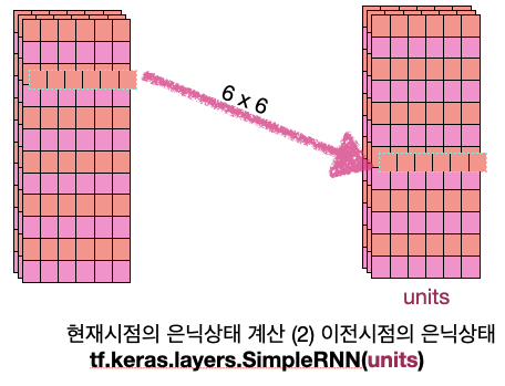
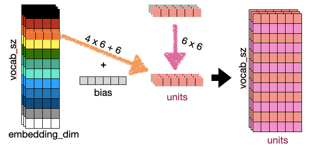
그리고 은닉층을 통과한 텐서는 위의 그림처럼 변환되게 된다. 이때 units 은 은닉층의 크기 를 의미한다. 은닉층의 파라미터는 아래 그림과 같다.
1번 그림의 vocab_sz는 sequence length인데 바꾸기가 귀찮았다. 여튼 내가 이해한 것은 이랬고, 결국 두개를 합쳐서 그려보면 아래와 같아진다.
중간의 (3, 6) 텐서가 현재시점의 은닉상태이다. 즉, hidden state의 shape은 (num of sequence, 은닉상태 크기) 이다.
Attention 1. 클래스 설계 1 2 3 4 5 6 7 8 9 10 11 12 13 14 15 16 17 18 19 20 21 22 23 24 25 26 27 28 class BahdanauAttention (tf.keras.layers.Layer ): def __init__ (self, units ): super (BahdanauAttention, self).__init__() self.W1 = tf.keras.layers.Dense(units) self.W2 = tf.keras.layers.Dense(units) self.V = tf.keras.layers.Dense(1 ) def call (self, query, values ): query_with_time_axis = tf.expand_dims(query, 1 ) score = self.V(tf.nn.tanh( self.W1(query_with_time_axis) + self.W2(values))) attention_weights = tf.nn.softmax(score, axis=1 ) context_vector = attention_weights * values context_vector = tf.reduce_sum(context_vector, axis=1 ) return context_vector, attention_weights
2. 사용 1 2 3 4 5 attention_layer = BahdanauAttention(10 ) attention_result, attention_weights = attention_layer(sample_hidden, sample_output) print ("Attention result shape: (batch size, units) {}" .format (attention_result.shape))print ("Attention weights shape: (batch_size, sequence_length, 1) {}" .format (attention_weights.shape))
Decoder 1. 클래스 설계 1 2 3 4 5 6 7 8 9 10 11 12 13 14 15 16 17 18 19 20 21 22 23 24 25 26 27 28 29 30 31 32 33 34 35 class Decoder (tf.keras.Model ): def __init__ (self, vocab_size, embedding_dim, dec_units, batch_sz ): super (Decoder, self).__init__() self.batch_sz = batch_sz self.dec_units = dec_units self.embedding = tf.keras.layers.Embedding(vocab_size, embedding_dim) self.gru = tf.keras.layers.GRU(self.dec_units, return_sequences=True , return_state=True , recurrent_initializer='glorot_uniform' ) self.fc = tf.keras.layers.Dense(vocab_size) self.attention = BahdanauAttention(self.dec_units) def call (self, x, hidden, enc_output ): context_vector, attention_weights = self.attention(hidden, enc_output) x = self.embedding(x) x = tf.concat([tf.expand_dims(context_vector, 1 ), x], axis=-1 ) output, state = self.gru(x) output = tf.reshape(output, (-1 , output.shape[2 ])) x = self.fc(output) return x, state, attention_weights
2. 사용 1 2 3 4 5 6 decoder = Decoder(vocab_tar_size, embedding_dim, units, BATCH_SIZE) sample_decoder_output, _, _ = decoder(tf.random.uniform((BATCH_SIZE, 1 )), sample_hidden, sample_output) print ('Decoder output shape: (batch_size, vocab size) {}' .format (sample_decoder_output.shape))
The optimizer and the loss function 1 2 3 4 5 6 7 8 9 10 11 12 optimizer = tf.keras.optimizers.Adam() loss_object = tf.keras.losses.SparseCategoricalCrossentropy( from_logits=True , reduction='none' ) def loss_function (real, pred ): mask = tf.math.logical_not(tf.math.equal(real, 0 )) loss_ = loss_object(real, pred) mask = tf.cast(mask, dtype=loss_.dtype) loss_ *= mask return tf.reduce_mean(loss_)
Checkpoints 1 2 3 4 5 checkpoint_dir = './training_checkpoints' checkpoint_prefix = os.path.join(checkpoint_dir, "ckpt" ) checkpoint = tf.train.Checkpoint(optimizer=optimizer, encoder=encoder, decoder=decoder)
Training 1 2 3 4 5 6 7 8 9 10 11 12 13 14 15 16 17 18 19 20 21 22 23 24 25 26 27 28 29 30 31 32 33 34 35 36 37 38 39 40 41 42 43 44 45 46 47 48 49 50 51 52 53 54 @tf.function def train_step (inp, targ, enc_hidden ): loss = 0 with tf.GradientTape() as tape: enc_output, enc_hidden = encoder(inp, enc_hidden) dec_hidden = enc_hidden dec_input = tf.expand_dims([targ_lang.word_index['<start>' ]] * BATCH_SIZE, 1 ) for t in range (1 , targ.shape[1 ]): predictions, dec_hidden, _ = decoder(dec_input, dec_hidden, enc_output) loss += loss_function(targ[:, t], predictions) dec_input = tf.expand_dims(targ[:, t], 1 ) batch_loss = (loss / int (targ.shape[1 ])) variables = encoder.trainable_variables + decoder.trainable_variables gradients = tape.gradient(loss, variables) optimizer.apply_gradients(zip (gradients, variables)) return batch_loss EPOCHS = 10 for epoch in range (EPOCHS): start = time.time() enc_hidden = encoder.initialize_hidden_state() total_loss = 0 for (batch, (inp, targ)) in enumerate (dataset.take(steps_per_epoch)): batch_loss = train_step(inp, targ, enc_hidden) total_loss += batch_loss if batch % 100 == 0 : print ('Epoch {} Batch {} Loss {:.4f}' .format (epoch + 1 , batch, batch_loss.numpy())) if (epoch + 1 ) % 2 == 0 : checkpoint.save(file_prefix = checkpoint_prefix) print ('Epoch {} Loss {:.4f}' .format (epoch + 1 , total_loss / steps_per_epoch)) print ('Time taken for 1 epoch {} sec\n' .format (time.time() - start))
![[딥러닝 스터디] Attention을 활용한 기계번역(실습)](/image/Elegant_Background-2.jpg)